Single precision

A run can hold its field and evaluate its nonlinear response in binary32 with precision="single", which halves the memory of every field-sized buffer. Whether a problem keeps its accuracy in binary32 is a property of the problem, so this example runs two of them both ways and compares: the photoionisation blue shift of Photoionisation-induced soliton blue-shift, here over its first 0.2 m, and a short radial argon filament, both on field grids with the field-grid plasma. Each runs in binary64 on the default backend, native, and in binary32 on the reference backend, numpy_ref, which is named explicitly: it is the backend that runs single precision.

What to look for. The two precisions’ output spectra lie on top of each other on a 40 dB scale; their difference, normwise over the whole saved field, is set by the controller’s tolerance and the binary32 propagator’s rounding, which accumulates over the run’s steps, and the energy, the spectral centroid, the electron density, the peak intensity and the beam radius agree to the digits printed. The printed times show the unthreaded reference’s binary32 run slower than native’s binary64 one: here single precision is a check of accuracy, not a speed-up (Single precision).

What is approximate. Single precision’s tolerance floor is rtol = 1e-6 (the default here); a problem that amplifies small perturbations strongly, such as a noise-free comb-to-continuum, reaches its accuracy over a shorter length, as the survival record states. Timings depend on the machine and its load.

The capillary, in both precisions

import time

import matplotlib.pyplot as plt
import numpy as np

from solprop.constants import C
from solprop.driver import Simulation, SimulationSettings, prop_capillary
from solprop.grid import FieldGrid, RadialGrid
from solprop.nonlinear.optmat_rates import OptmatRate
from solprop.nonlinear.responses import KerrResponse, PlasmaResponse
from solprop.physdata import gamma3
from solprop.processing import get_spectral_density
from solprop.pulses import GaussianPulse, SpatialPulse
from solprop.spatial import SpatialMedium, critical_power
from solprop.stepper import PIController

# Binary64 on the default backend, binary32 on the reference, the backend that runs it.
BACKENDS = {"double": "auto", "single": "numpy_ref"}


def capillary(precision):
    """Run the blue-shift capillary's first 0.2 m; return it and its time."""
    started = time.perf_counter()
    run = prop_capillary(
        13e-6,
        0.2,
        "Ar",
        1.7,
        wavelength=800e-9,
        fwhm=30e-15,
        energy=3e-6,
        loss=False,
        trange=600e-15,
        wavelength_limits=(300e-9, 4e-6),
        plasma=True,
        n_save=51,
        precision=precision,
        backend=BACKENDS[precision],
        progress="none",
        noise=None,
    )
    return run, time.perf_counter() - started


runs = {precision: capillary(precision) for precision in ("double", "single")}
for precision, (run, seconds) in runs.items():
    print(f"{precision}: {seconds:.1f} s on {run.metadata.backend.name}")


def relative(a, b):
    """Return the normwise relative difference of two arrays."""
    return float(np.linalg.norm(a - b) / np.linalg.norm(b))


double, single = runs["double"][0], runs["single"][0]
print(
    "field difference at the end "
    f"{relative(single.fields()[-1], double.fields()[-1]):.1e}"
)

double: 12.7 s on native
single: 99.6 s on numpy_ref
field difference at the end 8.9e-06

The spectra and the plasma

fig, (left, right) = plt.subplots(1, 2, figsize=(10.0, 3.6))
for precision, style in (("double", "-"), ("single", "--")):
    run = runs[precision][0]
    omega, spectral = get_spectral_density(run, "omega")
    keep = omega > 0
    wavelength = 2 * np.pi * C / omega[keep]
    level = spectral[-1, keep] / spectral[-1, keep].max()
    left.plot(
        wavelength * 1e9,
        10 * np.log10(np.maximum(level, 1e-6)),
        style,
        label=precision,
    )
    z = np.asarray(run["z"])
    density = np.asarray(run["stats/electron_density"]).reshape(z.size, -1).max(axis=1)
    right.plot(z, density * 1e-6, style, label=precision)
    centroid = 2 * np.pi * C * np.sum(spectral[-1]) / np.sum(spectral[-1] * omega)
    energy = float(np.asarray(run["stats/energy"]).ravel()[-1])
    print(
        f"{precision}: centroid {centroid * 1e9:.2f} nm, energy {energy * 1e6:.5f} uJ, "
        f"peak electron density {density.max() * 1e-6:.4e} cm^-3"
    )
left.set_xlim(300, 1600)
left.set_ylim(-40, 2)
left.set_xlabel("wavelength (nm)")
left.set_ylabel("spectral density at 0.2 m (dB)")
left.legend()
right.set_xlabel("z (m)")
right.set_ylabel("peak electron density (cm$^{-3}$)")
right.legend()
fig.tight_layout()

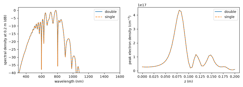
double: centroid 669.01 nm, energy 1.33141 uJ, peak electron density 4.3531e+17 cm^-3
single: centroid 669.01 nm, energy 1.33141 uJ, peak electron density 4.3531e+17 cm^-3

A radial filament, in both precisions

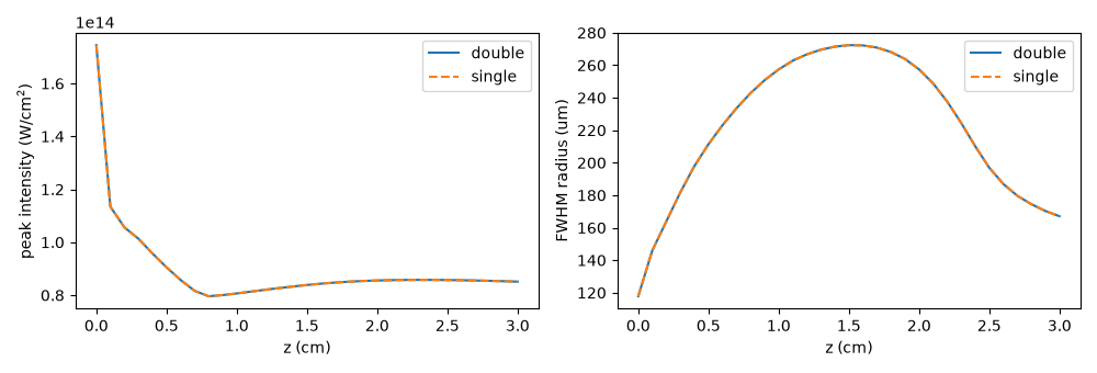
A 30 fs pulse at three times the critical power for self-focusing, 3 cm in argon at one bar, on 256 radial nodes in 2 mm and a field grid: Kerr self-focusing and the field-grid plasma on every node.

medium = SpatialMedium("Ar", 1.0)
chi3 = gamma3("Ar", wavelength=800e-9)
grid = FieldGrid.from_limits(0.03, 800e-9, (350e-9, 2e-6), 250e-15)
carrier = 2 * np.pi * C / 800e-9
density = float(medium.density(np.array([0.0]))[0])
index = float(np.real(medium.index(np.array([carrier]))[0]))
power = 3.0 * critical_power(800e-9, chi3 * density, index=index)
energy = power * 30e-15 * np.sqrt(np.pi / (4 * np.log(2)))
pulse = SpatialPulse(
    GaussianPulse(wavelength=800e-9, fwhm=30e-15, energy=energy), 100e-6
)
responses = [
    KerrResponse(chi3, thg=False),
    PlasmaResponse("Ar", OptmatRate("Ar", 800e-9)),
]
filaments = {}
for precision in ("double", "single"):
    started = time.perf_counter()
    filaments[precision] = Simulation.from_radial(
        grid,
        RadialGrid(2e-3, 256),
        medium,
        responses,
        pulse,
        settings=SimulationSettings(
            controller=PIController(rtol=1e-6, atol=0.0),
            dz_max=1e-3,
            dz_init=3e-5,
            save_planes=list(np.linspace(0.0, 0.03, 31)[1:]),
            ionisation_field_range=(1e7, 1e11),
            precision=precision,
            backend=BACKENDS[precision],
        ),
        noise=None,
    ).run()
    run = filaments[precision]
    print(
        f"{precision}: {time.perf_counter() - started:.1f} s on "
        f"{run.metadata.backend.name}"
    )
ends = [filaments[precision].fields()[-1] for precision in ("single", "double")]
print(f"field difference at 3 cm {relative(*ends):.1e}")

fig, (left, right) = plt.subplots(1, 2, figsize=(10.0, 3.4))
for precision, style in (("double", "-"), ("single", "--")):
    run = filaments[precision]
    z = np.asarray(run["z"])
    peak = np.asarray(run["stats/peak_intensity"]).ravel()
    radius = np.asarray(run["stats/fwhm_r"]).ravel()
    left.plot(z * 1e2, peak * 1e-4, style, label=precision)
    right.plot(z * 1e2, radius * 1e6, style, label=precision)
    print(
        f"{precision}: peak intensity {peak.max() * 1e-4:.4e} W/cm^2, "
        f"final FWHM radius {radius[-1] * 1e6:.3f} um"
    )
left.set_xlabel("z (cm)")
left.set_ylabel("peak intensity (W/cm$^2$)")
left.legend()
right.set_xlabel("z (cm)")
right.set_ylabel("FWHM radius (um)")
right.legend()
fig.tight_layout()

BoundaryWarning: the safety ramp has removed 1.47e-06 of the launch energy above the input noise's share: content reached the grid's outer wavenumbers; refine the transverse grid (SEP 40 section 5.3)
double: 1.9 s on native
BoundaryWarning: the safety ramp has removed 1.47e-06 of the launch energy above the input noise's share: content reached the grid's outer wavenumbers; refine the transverse grid (SEP 40 section 5.3)
single: 61.6 s on numpy_ref
field difference at 3 cm 7.5e-07
double: peak intensity 1.7445e+14 W/cm^2, final FWHM radius 167.043 um
single: peak intensity 1.7445e+14 W/cm^2, final FWHM radius 167.043 um